15 minutes could save you from having to understand conditional probability
02 Aug 2025
Tags: stats
I recently received some junk mail from a national insurance company, which touted: “Customers who save when they switch save an average of over $800”. OK, so how many didn’t save money, and how much more they were charged? At least it’s not as meaningless as the GEICO slogan: “15 minutes could save you 15% or more.” It could save you nothing. It could cause frogs to rain from the sky. Anything could happen in 15 minutes.
Seriously, though, first let’s acknowledge that the average annual car insurance premium is between $1,000 and $3,000 in the US, depending on the state.. At the high end, $800 divided by $3,000 is 27%, and it’s an even higher percent as premium decreases. I don’t pay a ton of attention to car insurance rates but this seems, well, unlikely to me. Maybe (over) $800 is lifetime savings, not annual. Or maybe there was something else hidden in the fine print. But let’s give them the benefit of the doubt.
Here’s a toy example. Let’s say out that \(n\) people received an insurance quote that saved \(x\), and \(m\) people received a quote that was more expensive by \(y\). Let’s understand \(x\) to be positive and \(y\) to be negative. Regardless of how huge \(m\) or \(y\) might be, the expected value over the positive values is still \(x\).
Let’s explore a scenario that’s a little more generous. Assume the random variable \(X\) has a normal distribution with a mean \(\mu\) and standard deviation \(\sigma > 0\), and additionally let \(c = \frac{\mu}{\sigma}\) be the coefficient of variation of that distribution. For consistency we’ll mostly look at \(\sigma\) and \(c\). Let \(p\) be the PDF of that distribution, defined the usual way. By the definition of the error function \(\operatorname{erf}\), The probability that \(X\) is positive is \(a = \frac{1}{2} \left(1 + \operatorname{erf} \left(\frac{c}{\sqrt{2}}\right)\right)\). The integral of the pdf is \(b = \int_0^\infty xp(x) dx = \frac{\sigma }{2} \left( \sqrt{\frac{2}{π}} \exp \left(-\frac{c^2}{2}\right) + c + c \operatorname{erf} \left(\frac{c}{\sqrt{2}}\right)\right)\), via a tedious integration by parts exercise I won’t repeat here. Furthermore, \(b = \frac{\sigma}{2} \left( \sqrt{\frac{2}{π}} \exp\left(-\frac{c^2}{2}\right) + 2ac\right)\). The mean of \(X\) given \(X>0\) is therefore \(E\left(X|X>0 \right) = \frac{b}{a}\), or, where \(\operatorname{erfc}(x) = 1 - \operatorname{erf} (x)\) is the complementary error function:
\[E\left(X|X>0 \right) = \frac{b}{a} = \sigma \left(c + \sqrt{\frac{2}{π}} \frac{\exp\left(-\frac{c^2}{2}\right)} {\operatorname{erfc} \left(-\frac{c}{\sqrt{2}}\right)} \right)\]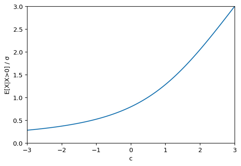
Above is a plot of \(\frac{E\left(X|X>0 \right)}{\sigma}\) as a function of \(c\). It looks like it approaches \(c\) as c approaches \(+\infty\), and approaches 0 as c approaches \(-\infty\) (although a lot more slowly). Let’s prove that. Note that \(\operatorname{erfc}(x)\) approaches 0 as \(x\) approaches \(+\infty\), that \(\operatorname{erfc}(x)\) approaches 2 as \(x\) approaches \(-\infty\), and that \(\operatorname{erfc}(0) = 1\). Let’s define \(m\) such that \(E\left(X|X>0 \right) = \sigma \left(c + m \right)\):
\[m=\sqrt{\frac{2}{π}} \frac{\exp\left(-\frac{c^2}{2}\right)} {\operatorname{erfc} \left(-\frac{c}{\sqrt{2}}\right)}\]As \(c\) approaches \(+\infty\), \(\exp\left(-\frac{c^2}{2}\right)\) approaches 0 while \(\operatorname{erfc} \left(-\frac{c}{\sqrt{2}}\right)\) approaches 2, so \(c\) approaches \(0\). We can also reason that if \(c\) is positive and large enough, then 0 is far away from the bulk of the distribution, and the \(X > 0\) condition doesn’t matter much.
The case where \(c\) approaches \(-\infty\) requires more work. To the Digital Library of Mathematical Functions! In 7.8.1, they define an auxilliary function for bounding purposes:
\[M(x) = \frac{\sqrt{\pi}}{2} \frac{\operatorname{erfc} (x)}{\exp (-x^2)}\]Inequality 7.8.5 (well, the outer part of it) is, when \(x \ge 0\),
\[\frac{x^2}{2x^2+1} \le x M(x) < \frac{x^2 + 1}{2x^2+3}\]Note that both bounds approach \(\frac{1}{2}\) as \(x\) approaches \(+\infty\), so the limit is \(x M(x) = \frac{1}{2}\). Substitute \(x = -\frac{c}{\sqrt{2}}\) and rearrange to get, as if by magic:
\[-c = \frac{1}{\sqrt{2} M\left(-\frac{c}{\sqrt{2}}\right)} = m\]Thus, the limit as \(c\) approaches \(-\infty\) is \(E\left(X|X>0 \right) = \sigma \left(c + m\right) = 0\). This seems reasonable: if \(c\) is a large negative, then the positive part of the distribution is just part of a thin tail, and most of it is near 0.
Finally, note that at \(c = 0\), \(E \left(X | X>0 \right) = \sigma \sqrt{\frac{2}{\pi}} \approx 0.8 \sigma\), which corresponds with the mean of the half-normal distribution, as expected.
Going back to the initial junk mail, if \(E\left(X|X>0 \right) = 800\), what does that say about \(c\) and \(\sigma\) (and therefore \(\mu\))? Well, the dividing line between positive and negative is \(c=\mu=0\), and from the last paragraph, we can back into a value for \(\sigma\) of about 1,000. Then let’s pick two convenient values for \(\sigma\) to test. \(\sigma = 400\) implies \(\frac{E\left(X|X>0 \right)}{\sigma} = 2\), which looking up from the graph earlier gives \(c \approx 1.98\). \(\sigma = 1600\) implies \(\frac{E\left(X|X>0 \right)}{\sigma} = 0.5\), which implies \(c \approx -1.08\). Of course these numbers are arbitrary, but it supports the suspicion that based on the number given in the junk mail, the real mean could reasonably be negative.
Anyways, the best advice I know is to go with whichever insurance company you can afford that has the best claims satisfaction, because it doesn’t matter how much you’re paying them if they won’t pay you when you need it.
(Hi! I’m not dead, I’m just got busy with the kind of work that actually pays me.)
Click here for the Python code to generate the plot above.
import numpy as np
import matplotlib.pyplot as plt
from scipy.special import erfc

x = np.linspace(-3,3,num=101)
y_c = x + np.exp(-x**2/2)*np.sqrt(2/np.pi)/erfc(-x/np.sqrt(2))

plt.plot(x, y_c)
plt.ylim(0,3)
plt.xlim(-3,3)
plt.xlabel('c')
plt.ylabel('E[X|X>0]')
plt.show()
Related Posts
- 2023-11-04: Spherical area coordinates, and a derived triangle center
- 2023-07-29: Homogeneous coordinates on the sphere with vectors
- 2022-08-30: Scaling the Schwarz triangle function
- 2022-08-27: Edges in the image of the Schwarz triangle function
- 2022-07-20: Area-preserving swirling of the disk
- 2022-03-03: Some dubious ways to calculate conformal polyhedral projections
- 2021-10-02: A variation on the Chamberlin trimetric map projection
- 2021-08-31: Snyder's equal-area projection
- 2021-06-12: Perspective projections with vectors
- 2021-05-29: A (sort of) Euclidean triangle on a non-Euclidean surface